FuryGpu’s Texture Units

Figure 1: FuryGpu Texture Unit
One of the most important aspects when it comes to rendering “realistic” images in games of the mid-to-late-90s (and even more so today!) is the replacement of geometric complexity with textures, where surface information and detail is encoded onto an image that is mapped onto the mesh by specifying sampling coordinates for each vertex. The stereotypical use case, at the time, was primarily focused on specifying the color of the mesh at a much higher resolution than would be possible through vertex coloring alone. Since FuryGpu is targeting features of this era, the ability to sample a texture for each rasterized pixel is a hard requirement. In addition, the relative cost associated with texture sampling (memory access, primarily) necessitates high clock rates, and caching to ensure that the act of sampling textures does not become a massive bottleneck.
At a high level, Texture Sampling (the operation performed by a Texture Unit) is a function of the desired texture and sampler specifications and the input texture coordinates. The texture specification tells the hardware the location of the texture in memory, its dimensions, its format, and anything else the texture unit requires to correctly turn a texel position into a color value. The sampler specification deals with the conversion from texture coordinates into texel positions and any filtering that needs to be performed on the resulting color values before they’re returned to the Rasterizer. The texture coordinates themselves I am going to assume should be self-explanatory to anyone reading a blog post about a custom GPU.
FuryGpu supports 2D texture sampling, power-of-two-dimensioned textures, variable numbers of mip levels, nearest and bilinear filtering (no trilinear!), and both raw RGBA8/RGB8 and color-tabled versions of those formats. These restrictions were necessary to reduce the amount of logic (and thus, increase the performance) of the texture unit as a whole, but are reasonably in-line with other GPU hardware of the era FuryGpu targets. Figure 1 shows the entire FuryGpu Texture Unit pipeline. This pipeline is instantiated once for each Rasterizer, as each gets its own Texture Unit. While the pipeline is per-Rasterizer, the AXI Masters are shared between them and typically operate on a first-come, first-serve basis. At the top and bottom of the pipeline, FIFOs are used to move requests into and results out. To try and minimize the impact that a textured draw call has versus a non-textured one, everything in the Texture Unit domain runs on a 480MHz clock (versus the 400MHz clock used by the rest of the GPU), necessitating CDC-enabled FIFOs. Unlike the Rasterizer pipeline, the Texture Unit is not pipelined such that it can accept and produce data every cycle. Instead, the various sub-modules use valid/ready signaling to move data between them in lockstep. With four sub-modules in the pipeline we can have four different sample requests active at any given time.
Each of the four Rasterizers in the GPU operates on a single primitive at a time, walking all 2x2 quads from the primitive that intersect the bounds of the tile being rendered and ensuring the pipeline is flushed before moving on to the next primitive. While this behavior does leave some performance on the table, it allows for the texture units to avoid having to keep track of the texture and sampler specifications for each stage of their pipelines, as only a single texture and sampler specification will be active at any given time. When a new primitive is prepared by a rasterizer, its texture and sampler information is moved into the associated texture unit. If the texture specification’s format includes a color table, the data for that table is read from memory into the color table BRAM, as well. The rasterization pipeline calculates the texture coordinates for each of the pixels in a given quad (including any that might not actually intersect the primitive - more on this later!) in fixed-point s16.16 format and passes those coordinates and a valid bit for each pixel in the quad through the Quad UVs Request FIFO. Passing a full 132 bits into a FIFO each cycle does take a fair amount of resources, but it is vital for keeping the pipelines as full as possible, as often as possible. Performance is the name of the game, here!
Reducing the effects of aliasing and increasing cache utilization by using mipmaps is a technique that has been used in GPUs (and computer graphics in general) for generations, and FuryGpu is no exception. This is why all the texture coordinates of all four pixels of each rasterized quad are sent through the request FIFO as a single unit; calculating texture coordinate derivatives in screen space requires the delta in both the X and the Y dimensions, and a 2x2 quad of coordinates gives us access to both. This calculation of the derivatives is the first operation performed in the Evaluate Texture LOD module in the pipeline, followed by the selection of the mip level that will be used when calculating texel addresses later. Modern GPUs use a rather complex mip-level selection function that takes into account the correct elliptical projection of the sampling region and involves a number of square roots and other arithmetic that would be far too costly to perform for our use case. Fortunately, a very reasonable estimation can be used instead and these equations can be simplified dramatically. Given the set of four input texture coordinates and the valid pixel bits, the LOD selection is performed as shown in the following pseudocode block. The pixels in the quad are specified in a Z ordering (index 0 is upper left, 1 is upper right, 2 is bottom left, 3 is bottom right).
// Select the row and column with the most valid pixels for the following calculations
valid_row = quad_valid[2] & quad_valid[3] ? 1 : 0;
valid_col = quad_valid[1] & quad_valid[3] ? 1 : 0;
row = valid_row ? {quad_uv[3], quad_uv[2]} : {quad_uv[1], quad_uv[0]};
col = valid_col ? {quad_uv[3], quad_uv[1]} : {quad_uv[2], quad_uv[0]};

// Compute the absolute value of the difference between the rows and columns
// giving the change in texture coordinates with respect to screen coordinates
ddx = abs({row[1].y - row[0].y, row[1].x - row[0].x});
ddy = abs({col[1].y - col[0].y, col[1].x - col[0].x});

// Scale the derivatives by the dimensions of the base mip level
// Since we only support powers of two dimensions, this is a simple left shift
ddx = ddx << {height_pot, width_pot};
ddy = ddy << {height_pot, width_pot};

// Find the largest of the squared ddx and ddy
d = max(dot(ddx, ddx), dot(ddy, ddy));

// Since we do not support trilinear filtering, we only need the integer part of the log2
lod = min((16 - lzc(d)) / 2, max_lod);
Mip LOD selection takes 11 cycles, four of which are pipelining for the DSP multiplications used in the dot product calculations.
Following mip LOD selection, the LOD index and the original input texture coordinates are passed through to the Texture Coordinate Evaluation sub-module to determine the image texel indices for the texels that influence each pixel in the quad are read. Texture coordinate inputs from the Rasterizer are normalized, with the [0, 1] range mapped to the full extent of the texture image. At this point in the pipeline, the addressing modes for the U and V dimensions defined in the Sampler specification are used to determine how texture coordinates that fall outside of the normalized range are handled. FuryGpu supports three addressing modes: wrap, clamp, and mirror. The Wrap mode repeats the image, allowing it to tile multiple times; the Clamp mode clamps the coordinates to the [0, 1] range, causing the edge texels to repeat; the Mirror mode behaves like Wrap, but flips the image for the odd tilings. Applying the addressing modes re-normalizes the texture coordinates, which are then scaled by the dimensions of the mip level selected in the previous stage. This gives us an absolute texel coordinate for each valid pixel in the quad.
At this point, we have the mip level to sample from and the texel coordinates inside that mip, so the next step is to figure out the actual memory address that can be read from to return that specific texel’s data. With a naive approach, this operation would involve having to iterate through the mip levels to figure out the offset from the base address of the texture for the specific one we’re interested in; textures do have power-of-two dimensions, but they are not necessarily square. Having to do this iteration at runtime would require a significant amount of logic (the hardware would have to exist for the worst-case number of iterations!) and would take dozens of additional cycles. Doing things this way would not allow FuryGpu to meet its performance goals, so a different method is needed. Fortunately, the UltraScale+ FPGA FuryGpu is built on has ample BRAM resources that can be configured as ROMs with pre-defined contents. With some clever data layout and a simple Python script, we can fit the memory offset from the texture base address for all possible mip levels of all possible texture dimensions into a pair of ROMs, from which we can read that offset in just two cycles. By limiting the dimensions to 2^11 (2048x2048), storing the mip levels from smallest to largest (reducing the maximum offset by the size of the largest possible mip), and enforcing a minimum memory size per mip of 16 texels, the largest offset we need to store can fit into exactly 18 bits. Each ROM is thus set up as 4K entries of 9 bits, which fits perfectly into the 36Kb BRAMs on the device. The following Python script is used to generate the data for these ROMs, the output of which is split into two 9-bit data streams that are used to initialize the ROMs when the design is synthesized.
offsets = []
# Gotta iterate from MSB to LSB, so the indices are sequential
for log2_width in range(16):
    for log2_height in range(16):
        for mip in range(16):
            offset_idx = log2_width*16*16 + log2_height*16 + mip

            width = 1 << log2_width
            height = 1 << log2_height

            offset = 0

            num_mips = max(log2_width, log2_height) + 1
            if log2_width < 12 and log2_height < 12 and mip < 13 and mip < num_mips:
                # Begin summing up the offset for this mip for the given width and height
                # Note that we store the mips backwards, so mip 0 has the largest offset!
                for cur_mip in range(num_mips-1, mip, -1):
                    log2_cur_mip_width = max(log2_width - cur_mip, 2)
                    log2_cur_mip_height = max(log2_height - cur_mip, 2)

                    # Divide by 16, which is the smallest increment we can have
                    cur_size = 1 << (log2_cur_mip_width + log2_cur_mip_height - 4)
                    offset += cur_size
            else:
                # Fill the invalid regions of the ROM with all 1s
                offset = (1 << 18) - 1

            #print('{0}x{1} mip {2}: {3}'.format(width, height, mip, offset))
            offsets.append(offset)
In this stage of the pipeline, we’ve also broken the quad apart into individual pixels, and only the valid pixels move on to the next stage, which is by far the most simple in the pipeline: Calculate Texel Address!
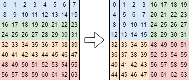
Figure 2: Texel Tiling
For each valid texel that makes it to this stage, the only thing we have to do here is determine the final memory address corresponding to the texel. This depends on the texture format (different formats have different-size texels) and whether or not the texture is using a color table (in which case the mips start after the color table data). Additionally, the texels are reordered in memory (“tiled”) into 4x4 blocks of texels as shown in Figure 2. Performing this tiling improves the likelihood that texels that are likely to be sampled by neighboring pixels (and the neighboring texels when performing bilinear filtering) will end up sharing the same cache line, reducing the memory access cost dramatically. If the Sampler specification indicates bilinear filtering is to be used, the initial texel address as well as the addresses for the three surrounding texels that will be used as part of the filter are calculated. For nearest filtering, only the initial texel address is determined. The final texel addresses are emitted from this stage and enter the Texel Filtering sub-module.
Before getting into how the Texel Filtering sub-module works, it is worth spending some time discussing the way that the Texture Unit tries to avoid the most expensive operation involved in the entire process: memory access. Since the AXI4 bus used for texel memory access connects directly to the hardened DDR3 memory controller in the ZynqMP, any read request is going to take the full DDR3 access time - potentially hundreds of cycles. To mitigate this as much as possible, each Texture Unit contains a Texture Cache that reduces that cost down to roughly ten cycles on a cache hit and just a single cycle on a repeated read from the same cache line.

Figure 3: Texture Cache Block Diagram
The Texture Cache is implemented as a read-through, four-way, set-associative cache with a depth of 4096 elements utilizing 128-bit cache lines (matching the width of the AXI4 bus). This cache line size also reflects the size of each 4x4 tile when using a color-mapped texture format, which means that it is extremely common for nearby texture samples to end up pulling directly from the same cache line. Four ways and 4096 elements in the cache comes out to 1024 sets, giving the following constants and calculations for the width of the tag necessary to identify the cache lines stored in the cache:
localparam CACHE_LINE_WIDTH = 128;
localparam CACHE_LINE_ADDR_LSB = $clog2(CACHE_LINE_WIDTH / 8);			// 4
localparam CACHE_DEPTH = 4096;
localparam NUM_WAYS = 4;
localparam NUM_SETS = CACHE_DEPTH / NUM_WAYS;					// 1024
localparam SET_IDX_WIDTH = $clog2(NUM_SETS);					// 10
localparam ADDR_WIDTH = 31;								// 2GB of accessible VRAM fits in 31 bits!
localparam TAG_WIDTH = ADDR_WIDTH - SET_IDX_WIDTH - CACHE_LINE_ADDR_LSB;	// 17
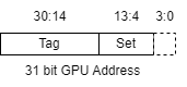
Figure 4: Address Set/Tag
Along with an additional valid bit, each tag takes up 18 bits of space. These numbers are extremely fortunate given the hardware we have to work with! 128 bit cache lines times 4096 entries in the cache puts us at 512Kb of cache, which we can fit into a pair of 288Kb UltraRAM blocks utilizing all of their available depth with each configured as 4K*64 (256Kb). Likewise, the tag data for the 1024 sets in each of the four ways can fit into a pair of 36Kb BRAMs configured as 2K*18 (36Kb). Utilizing both ports on each BRAM allows reading of the tag data for all ways of a given set simultaneously, making it extremely fast to perform these lookups as will soon see outlined in the following pseudocode demonstrating a cache query.
if (prev_cache_query_addr == query_addr) begin
    return prev_cache_line;
end

addr_set = query_addr[CACHE_LINE_ADDR_LSB+:SET_IDX_WIDTH];
addr_tag = query_addr[ADDR_WIDTH-1:SET_IDX_WIDTH+CACHE_LINE_ADDR_LSB];

hit = {false, false, false, false};
hit_way_idx = -1;
for (i = 0; i < 4; ++i) begin
    // vtag_bram is really just two BRAMs (not four), each split in half
    vtag = vtag_bram[i][addr_set];
    if (vtag.valid && vtag.tag == addr_tag) begin
        hit_way_idx = i;
        hit[i] = true;
    end
end

if (any(hit)) begin
    cache_line = cache_line_uram[{addr_set, hit_way_idx}];
    // Mark the opposite pair of ways as the LRU for the eviction strategy
    lru_bram[addr_set] = ~hit_way_idx[1];
end else begin
    cache_line = ReadCacheLineFromMemory(query_addr);
    lru_way_msb = lru_bram[addr_set];
    // If any of the ways for the set are not valid, use one of those; otherwise, pick
    // the least recently used pair of ways and a pseudo-random way in that set
    target_way_idx = ~all(hit) ? FirstFalseIndex(hit) : {lru_way, one_bit_per_cycle_counter};
    cache_line_uram[{addr_set, target_way_idx}] = cache_line;
end

// Save off the most recent cache line for one-cycle lookup if we query it again
prev_cache_query_addr = query_addr;
prev_cache_line = cache_line;

return cache_line;
Keeping track of the last cache line accessed through the cache and taking into account the 4x4 tiling performed on the texture data, we frequently end up hitting the same cache line for many of the cache lookups performed, returning the cache line immediately. In other cases, the full cache query behavior is performed. The tags stored in the four ways for the set of the address being queried are examined for validity and whether or not they match the query tag. In hardware, all four of these lookups and tag tests are performed simultaneously and have a four-cycle latency. A hit following this lookup immediately kicks off the correct read of the cached data, which is another four cycles. A miss initiates an AXI read of the desired cache line from memory, followed by an insertion of the cache line into the cache. This process can take upwards of a hundred cycles, as it requires access to the DDR3 memory. Since the entire Texture Unit pipeline requires that sample results return in the same order as requests were added, the entire pipeline unfortunately must be stalled during this memory access. A pseudo-least-recently-used eviction strategy is used to determine which way of the set will be replaced when all four contain valid data: each time a query has a valid hit on a given way, that way and its neighbor are marked as the most recently used pair of ways for that set. Additionally, a single bit register is toggled every cycle regardless of what else is going on in the cache. When it comes time to evict one of the ways of a set, the LRU bit and the toggled per-cycle bit are combined into a two-bit index to specify which way will be replaced in that set.

Figure 5: Bilinear Filter
With the cache out of the way, let’s get into why it exists in the first place. We left the pipeline at the point where either one or four texel addresses were exported from the Calculate Texel Addresses sub-module for each valid pixel in the quad. With the help of the Texture Cache, we now need to read the actual texel data from VRAM for each of those addresses. For raw RGB/RGBA texture formats, reading the texel data is as simple as reading the cache line they are part of and pulling out the desired bytes. Color-tabled formats use one byte per texel, and in order to find the actual texel information a given color index maps to, a lookup from the Color Table BRAM is performed. If the Sampler specification indicates nearest filtering, at this point the sampling process is complete and the results for the pixel quad are returned to the Rasterizer through the Sample Result FIFO. For bilinear filtering, an additional filtering pipeline stage is utilized to combine the four neighboring samples for each sampled texel and the precise sub-texel offset of the sample point into a single, filtered sample.

Figure 6: Dual 8-bit Color Multiply
The bilinear filtering equation itself is quite simple: a pair of linear interpolations between the samples of each row in the 2x2 quad of samples, followed by a linear interpolation between those two results. As seen in Figure 5, this boils down to simply f(α, β) = lerp(lerp(s0, s1, α), lerp(s2, s3, α), β) where α is the horizontal position of the sample point between texel centers and β is the vertical. A naive implementation of this process would require a significant number of multiplies (four color channels times two multiplies per lerp comes out to 24 multiplies!), but thanks to the wide 27x18 bit DSP48E2 multipliers on the UltraScale+ architecture, we can do better. Each color channel being interpolated is eight bits wide, and is being multiplied by an eight bit interpolation alpha value. Since the width of the first input to the DSP’s multiplier is 27 bits wide, we can place two color values at opposite ends of that vector (taking into account that the multiplier is signed, so we need to avoid using the MSB to keep it fixed at zero!), and then place the interpolation alpha in the second input to give us two multiplies for the price of one as shown in Figure 6. With this technique, we cut the number of required multiplication operations down to just 12. Additionally, the scalar lerp operation is defined as lerp(x, y, a) = (1-a)*x + a*y, which can be rewritten as x - a*x - a*y, removing the dependency of the calculation of 1-a and allowing both multiplications to be performed against the same multiplicand. Using this formulation of the lerp operation, we can perform all the multiplications for the initial horizontal row lerps at the same time, followed by the remaining lerp immediately thereafter. With this setup, a fully pipelined bilinear filtering is performed in just eight cycles.
Finally, the sample results for each valid pixel of the input quad are packed back together and returned to the Rasterizer through another CDC FIFO, and the texture sampling process is complete. All together, FuryGpu’s four Texture Unit pipelines consume 9419 LUTs, 23075 FFs, 18 BRAMs, 8 URAMs, and 76 DSPs. Clocked at 480MHz, the Texture Unit is the most deeply pipelined portion of the entire GPU - absolutely necessary to meet timing at this clock rate!